Preparing your data for MIDAS#

This tutorial walks through preparing a single-cell multi-modal dataset for MIDAS, starting from a publicly downloadable 10x Genomics CITE-seq sample (~5 200 cells, RNA + 32 antibodies). The pipeline is built on scanpy and produces a :class:MuData ready to pass to :class:scmidas.MIDAS.

The same recipe scales to your own data: replace the download cell with how you load your AnnData(s) and the rest of the steps are identical.

In a hurry? If you just want to use MIDAS, skip this notebook entirely and run any of the bundled tutorials in docs/source/tutorials/basics/. They use already-preprocessed datasets so you can focus on the model.

Looking for the original preprocessing pipeline? The reproducibility branch (with docs) contains the scripts used in the manuscript across multiple tissues and modality combinations (PBMC CITE-seq, bone marrow, TEA-seq, multiome). The bundled demo1 / demo2 / demo3 datasets were produced from those scripts and may differ slightly from the manuscript figures because the source data has been updated since publication. The scanpy pipeline below is a self-contained alternative for getting started on your own data — it is not a re-implementation of those scripts.

What you’ll learn:

Downloading a 10x CITE-seq sample (1 line)
Standard scanpy QC (mt%, count thresholds, doublet-aware)
Per-modality normalization choices and HVG selection
Wrapping per-modality AnnDatas as :class:MuData with the contract MIDAS expects
Running MIDAS end-to-end and a tiny scanpy downstream (Leiden + UMAP)
(Bonus) Synthesizing a mosaic MuData from a single dataset, so you can see the layout the demos use

1. Setup#

[1]:

import warnings
warnings.filterwarnings('ignore')
import logging
logging.basicConfig(level=logging.INFO)

from pathlib import Path
import urllib.request

import anndata as ad
import lightning as L
import matplotlib.pyplot as plt
import mudata as mu
import numpy as np
import pandas as pd
import scanpy as sc

import scmidas

sc.set_figure_params(figsize=(4, 4))
L.seed_everything(42, verbose=False)

[1]:

2. Download a public CITE-seq dataset#

We use the 5k PBMC protein v3 sample from 10x Genomics — a healthy-donor PBMC CITE-seq with ~5 200 cells, paired RNA (~33k genes) and 32 antibody capture (ADT) features. The filtered .h5 is ~17 MB.

[2]:

DATA_DIR = Path('dataset/_pbmc5k_demo')
DATA_DIR.mkdir(parents=True, exist_ok=True)
H5 = DATA_DIR / '5k_pbmc_protein_v3_filtered_feature_bc_matrix.h5'

if not H5.exists():
    import requests
    url = (
        'https://cf.10xgenomics.com/samples/cell-exp/3.0.2/5k_pbmc_protein_v3/'
        '5k_pbmc_protein_v3_filtered_feature_bc_matrix.h5'
    )
    print(f'Downloading {url} ...')
    r = requests.get(url, headers={'User-Agent': 'Mozilla/5.0'}, stream=True)
    r.raise_for_status()
    with open(H5, 'wb') as f:
        for chunk in r.iter_content(chunk_size=1 << 20):
            f.write(chunk)
print(f'  size: {H5.stat().st_size / 1e6:.1f} MB')

# 10x's CITE-seq h5 packs RNA + antibody capture in one matrix.
adata_all = sc.read_10x_h5(H5, gex_only=False)
adata_all.var_names_make_unique()
print(adata_all)
print('feature_types:', adata_all.var['feature_types'].value_counts().to_dict())

  size: 17.1 MB
AnnData object with n_obs × n_vars = 5247 × 33570
    var: 'gene_ids', 'feature_types', 'genome', 'pattern', 'read', 'sequence'
feature_types: {'Gene Expression': 33538, 'Antibody Capture': 32}

3. Split RNA and ADT into separate AnnData objects#

This step is generic 10x Genomics handling. It isnotMIDAS-specific.

MIDAS expects one :class:AnnData per modality. Splitting now also lets each modality go through its own QC and normalization.

[3]:

is_rna = adata_all.var['feature_types'] == 'Gene Expression'
is_adt = adata_all.var['feature_types'] == 'Antibody Capture'

adata_rna = adata_all[:, is_rna].copy()
adata_adt = adata_all[:, is_adt].copy()

print(f'RNA: {adata_rna.shape}, ADT: {adata_adt.shape}')

RNA: (5247, 33538), ADT: (5247, 32)

4. Per-modality QC#

This step isstandard scanpy QC(mt%, gene/count thresholds), applied per modality.

The thresholds below mirror those used in the MIDAS paper’s R/Seurat preprocessing. Pick your own thresholds for your own data — these are reasonable defaults for 10x PBMC.

[4]:

# RNA QC: count + gene + mt% thresholds
adata_rna.var['mt'] = adata_rna.var_names.str.startswith('MT-')
sc.pp.calculate_qc_metrics(
    adata_rna, qc_vars=['mt'], percent_top=None, log1p=False, inplace=True,
)

keep_rna = (
    (adata_rna.obs['n_genes_by_counts'].between(500, 6000)) &
    (adata_rna.obs['total_counts'].between(600, 40000)) &
    (adata_rna.obs['pct_counts_mt'] < 15)
)

# ADT QC: count thresholds only
sc.pp.calculate_qc_metrics(adata_adt, percent_top=None, log1p=False, inplace=True)
keep_adt = adata_adt.obs['total_counts'].between(400, 20000)

# Keep cells that pass BOTH modality QCs (intersection).
keep = keep_rna & keep_adt
print(f'Cells passing RNA QC: {int(keep_rna.sum())}/{len(keep_rna)}')
print(f'Cells passing ADT QC: {int(keep_adt.sum())}/{len(keep_adt)}')
print(f'Cells passing BOTH:   {int(keep.sum())}/{len(keep)}')

adata_rna = adata_rna[keep].copy()
adata_adt = adata_adt[keep].copy()

Cells passing RNA QC: 4031/5247
Cells passing ADT QC: 5215/5247
Cells passing BOTH:   4013/5247

5. Highly-variable genes for RNA#

Generic scanpy. ADT keeps all features (only ~30 antibodies — no need to subset).

MIDAS reads raw count data and applies its own internal log1p transform during the forward pass (controlled by the trsf_before_enc_rna config). So we subset by HVG but keep raw counts — do not call sc.pp.normalize_total or sc.pp.log1p here.

[5]:

# scanpy's seurat-v3 HVG flavor needs scikit-misc; avoid that extra dep
# by using the classic flow: keep a copy of raw counts, normalize,
# log1p, run HVG, then restore raw counts on the subsetted AnnData.
# MIDAS wants raw counts (it applies its own log1p internally).
import scipy.sparse as sp

raw_counts = adata_rna.X.copy()
raw_var_names = adata_rna.var_names.copy()

sc.pp.normalize_total(adata_rna, target_sum=1e4)
sc.pp.log1p(adata_rna)
sc.pp.highly_variable_genes(adata_rna, n_top_genes=4000, flavor='seurat')

hvg_mask = adata_rna.var['highly_variable'].values
adata_rna = adata_rna[:, hvg_mask].copy()
col_idx = [raw_var_names.get_loc(g) for g in adata_rna.var_names]
adata_rna.X = raw_counts[:, col_idx]

print(f'RNA after HVG: {adata_rna.shape}')
print(f'ADT (kept all): {adata_adt.shape}')

RNA after HVG: (4013, 4000)
ADT (kept all): (4013, 32)

6. Wrap as a MuData with the MIDAS contract#

This is theMIDAS-specificpart — and it’s the only step that’s not pure scanpy.

The contract is small:

One AnnData per modality, with .X holding raw counts (or whatever the model’s trsf_before_enc_* config expects).
A ``batch`` column (or any name you want, passed via batch_key later) in each modality’s .obs. It identifies the source batch / donor / sample. Even with one batch, this column must exist.
Consistent ``obs_names`` between modalities for cells that have both — this is how MIDAS knows the cells are paired.

For our single-donor sample, we just label everything 'donor_a'.

[6]:

adata_rna.obs['batch'] = 'donor_a'
adata_adt.obs['batch'] = 'donor_a'

mdata = mu.MuData({'rna': adata_rna, 'adt': adata_adt})
print(mdata)

MuData object with n_obs × n_vars = 4013 × 4032
  var:  'gene_ids', 'feature_types', 'genome', 'pattern', 'read', 'sequence', 'n_cells_by_counts', 'mean_counts', 'pct_dropout_by_counts', 'total_counts'
  2 modalities
    rna:        4013 × 4000
      obs:      'n_genes_by_counts', 'total_counts', 'total_counts_mt', 'pct_counts_mt', 'batch'
      var:      'gene_ids', 'feature_types', 'genome', 'pattern', 'read', 'sequence', 'mt', 'n_cells_by_counts', 'mean_counts', 'pct_dropout_by_counts', 'total_counts', 'highly_variable', 'means', 'dispersions', 'dispersions_norm'
      uns:      'log1p', 'hvg'
    adt:        4013 × 32
      obs:      'n_genes_by_counts', 'total_counts', 'batch'
      var:      'gene_ids', 'feature_types', 'genome', 'pattern', 'read', 'sequence', 'n_cells_by_counts', 'mean_counts', 'pct_dropout_by_counts', 'total_counts'

7. Run MIDAS end-to-end#

MIDAS-specific. This is the same ``scmidas.integrate`` you’d use on multi-batch data.

scmidas.integrate(...) is a one-call wrapper that calls setup_mudata, constructs the model, trains, and writes the joint biological latent to mdata.obsm['X_midas']. With a single-donor 5k-cell dataset, training takes ~1 min on a mid-range GPU.

Single-donor data has no batch effect to correct, so this run is mainly a sanity-check that the data layout is valid. For a meaningful integration you’d combine multiple datasets / donors with the same MuData structure (see the demos in docs/source/tutorials/basics/).

[7]:

model = scmidas.integrate(mdata, batch_size=128, max_epochs=100)

print('mdata.obsm[X_midas].shape =', mdata.obsm['X_midas'].shape)

INFO:scmidas.config:The model is initialized with the default configurations.
INFO:scmidas.api:scmidas.integrate(): toy-tuned defaults — batch_size=128, max_epochs=100, lr=0.0003. For real datasets, override max_epochs (e.g. 2000) and consider batch_size=256.
INFO:scmidas.model:setup_mudata: batch_key='batch', batches=['donor_a'], modalities=['rna', 'adt'], dims_x={'rna': [4000], 'adt': [32]}
INFO:scmidas.model:Input data:
         #CELL  #RNA  #ADT
donor_a   4013  4000    32
INFO: 💡 Tip: For seamless cloud uploads and versioning, try installing [litmodels](https://pypi.org/project/litmodels/) to enable LitModelCheckpoint, which syncs automatically with the Lightning model registry.
INFO:lightning.pytorch.utilities.rank_zero:💡 Tip: For seamless cloud uploads and versioning, try installing [litmodels](https://pypi.org/project/litmodels/) to enable LitModelCheckpoint, which syncs automatically with the Lightning model registry.
INFO: GPU available: True (cuda), used: True
INFO:lightning.pytorch.utilities.rank_zero:GPU available: True (cuda), used: True
INFO: TPU available: False, using: 0 TPU cores
INFO:lightning.pytorch.utilities.rank_zero:TPU available: False, using: 0 TPU cores
INFO: HPU available: False, using: 0 HPUs
INFO:lightning.pytorch.utilities.rank_zero:HPU available: False, using: 0 HPUs
INFO: LOCAL_RANK: 0 - CUDA_VISIBLE_DEVICES: [0,1,2,3,4,5,6,7]
INFO:lightning.pytorch.accelerators.cuda:LOCAL_RANK: 0 - CUDA_VISIBLE_DEVICES: [0,1,2,3,4,5,6,7]
INFO:
  | Name | Type          | Params | Mode
-----------------------------------------------
0 | net  | VAE           | 8.5 M  | train
1 | dsc  | Discriminator | 38.8 K | train
-----------------------------------------------
8.6 M     Trainable params
0         Non-trainable params
8.6 M     Total params
34.350    Total estimated model params size (MB)
144       Modules in train mode
0         Modules in eval mode
INFO:lightning.pytorch.callbacks.model_summary:
  | Name | Type          | Params | Mode
-----------------------------------------------
0 | net  | VAE           | 8.5 M  | train
1 | dsc  | Discriminator | 38.8 K | train
-----------------------------------------------
8.6 M     Trainable params
0         Non-trainable params
8.6 M     Total params
34.350    Total estimated model params size (MB)
144       Modules in train mode
0         Modules in eval mode
INFO:scmidas.model:Total number of samples: 4013 from 1 datasets.
INFO:scmidas.model:Using MultiBatchSampler for data loading.
INFO:scmidas.model:DataLoader created with batch size 128 and 20 workers.

INFO: `Trainer.fit` stopped: `max_epochs=100` reached.
INFO:lightning.pytorch.utilities.rank_zero:`Trainer.fit` stopped: `max_epochs=100` reached.
INFO:scmidas.model:Checkpoint successfully saved to "./saved_models/scmidas/model_epoch100_20260509-031133.pt".

mdata.obsm[X_midas].shape = (4013, 32)

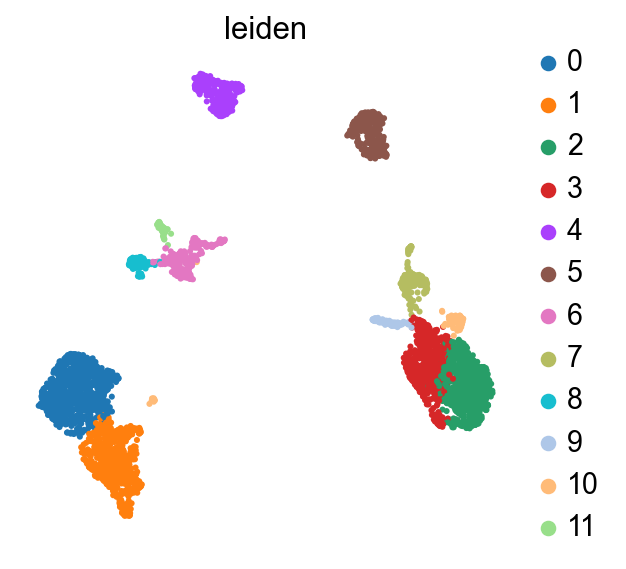
8. scanpy-native downstream — Leiden + UMAP#

Generic scanpy. Everything scmidas.integrate produced lives in mdata.obsm['X_midas'], so any tool that takes a use_rep= argument works out of the box.

Below we cluster with Leiden, plot the UMAP coloured by cluster, and show how to start hand-annotating cell types from marker genes (or, if you want full automation, drop in `celltypist <https://www.celltypist.org/>`__ here).

[8]:

# Build a temporary AnnData wrapping X_midas so we can use the full
# scanpy downstream stack. The result (Leiden labels) is copied back
# to mdata.obs so plotting helpers see it.
ad_view = ad.AnnData(X=mdata.obsm['X_midas'], obs=mdata.obs.copy())
sc.pp.neighbors(ad_view, use_rep='X', n_neighbors=15)
sc.tl.leiden(ad_view, resolution=0.5)
mdata.obs['leiden'] = ad_view.obs['leiden'].values

# Plot the UMAP coloured by Leiden cluster.
scmidas.pl.umap(
    mdata, basis='X_midas',
    color=['leiden'], frameon=False,
)

../../_images/tutorials_basics_preparing_your_data_16_0.png

[8]:

AnnData object with n_obs × n_vars = 4013 × 32
    obs: 'leiden'
    uns: 'neighbors', 'umap', 'leiden_colors'
    obsm: 'X_umap'
    obsp: 'distances', 'connectivities'

For automated cell-type labelling, CellTypist takes the same mdata['rna'] AnnData and predicts immune cell types from a pre-trained model. We don’t run it here to keep dependencies minimal, but a one-liner like:

# pip install celltypist
import celltypist
preds = celltypist.annotate(adata_rna, model='Immune_All_Low.pkl')
mdata.obs['celltypist'] = preds.predicted_labels.predicted_labels.values

drops cell-type names directly into mdata.obs.

9. Bonus — building a mosaic MuData (for understanding)#

The demos in docs/source/tutorials/basics/ integrate mosaic data: different batches contain different subsets of modalities (e.g. some batches have RNA only, some have ADT only, some have both). This section shows how the layout looks, by artificially splitting the single-donor data into three pseudo-batches with different modality availability.

This is for understanding the layout, not for real analysis: there is no genuine batch effect within a single donor.

[9]:

rng = np.random.default_rng(42)
n = adata_rna.n_obs
idx = rng.permutation(n)
i1, i2 = n // 3, 2 * n // 3
ids_b1, ids_b2, ids_b3 = idx[:i1], idx[i1:i2], idx[i2:]

# b1: RNA only; b2: ADT only; b3: paired RNA+ADT
ad_rna_b1 = adata_rna[ids_b1].copy(); ad_rna_b1.obs['batch'] = 'b1'
ad_rna_b3 = adata_rna[ids_b3].copy(); ad_rna_b3.obs['batch'] = 'b3'
ad_adt_b2 = adata_adt[ids_b2].copy(); ad_adt_b2.obs['batch'] = 'b2'
ad_adt_b3 = adata_adt[ids_b3].copy(); ad_adt_b3.obs['batch'] = 'b3'

# Concatenate per-modality across batches that have that modality.
ad_rna_all = ad.concat([ad_rna_b1, ad_rna_b3], join='outer')
ad_adt_all = ad.concat([ad_adt_b2, ad_adt_b3], join='outer')

mdata_mosaic = mu.MuData({'rna': ad_rna_all, 'adt': ad_adt_all})

print(mdata_mosaic)
print('per-modality batch counts:')
print('  rna:', dict(ad_rna_all.obs['batch'].value_counts()))
print('  adt:', dict(ad_adt_all.obs['batch'].value_counts()))

MuData object with n_obs × n_vars = 4013 × 4032
  2 modalities
    rna:        2675 × 4000
      obs:      'n_genes_by_counts', 'total_counts', 'total_counts_mt', 'pct_counts_mt', 'batch'
    adt:        2676 × 32
      obs:      'n_genes_by_counts', 'total_counts', 'batch'
per-modality batch counts:
  rna: {'b3': 1338, 'b1': 1337}
  adt: {'b2': 1338, 'b3': 1338}

You can now pass mdata_mosaic to scmidas.MIDAS.setup_mudata and scmidas.MIDAS(...); MIDAS will infer the mosaic structure (which batches lack which modalities) automatically. See demo2.ipynb for the same idea on a real 8-batch RNA+ADT dataset.

Where to go next#

Demo notebooks (docs/source/tutorials/basics/) walk through MIDAS on three preprocessed datasets, with mosaic and tri-modal cases.
Quickstart (examples/quickstart.ipynb) is the 5-line “does this work” path with the bundled toy data.
Reproducibility branch (github, docs) contains the original preprocessing scripts spanning the tissues and modality combinations used in the manuscript, including ATAC peak calling and batch-aware HVG selection.

For an even shorter pipeline (single-cell, single-modality preprocessing), refer to the standard scanpy Preprocessing and clustering tutorial — every step before “wrap as MuData” is the same.

Preparing your data for MIDAS

Contents