Mosaic Integration of RNA+ADT

In this tutorial, we demonstrate how to use MIDAS to integrate a mosaic dataset consisting of paired and unpaired RNA (gene expression) and ADT (antibody-derived tags) data.

1. Setting Up the Environment

We import the necessary libraries and set up the environment. The first code cell exposes a small GPU configuration block — GPUS and STRATEGY — that controls which device(s) the demo uses. The defaults run on a single GPU; switching to multi-GPU only requires changing those two values (see the comments inside that cell).

import warnings
warnings.filterwarnings('ignore')
import logging
logging.basicConfig(level=logging.INFO)
import os

# === GPU configuration ===
# Single-GPU (default; works inside this notebook):
GPUS = '0'
STRATEGY = 'auto'

# Multi-GPU options (uncomment one):
# - In a notebook (slower DDP startup, no script conversion needed):
#       GPUS = '0,1'; STRATEGY = 'ddp_notebook'
# - As a script (recommended for production multi-GPU):
#       GPUS = '0,1'; STRATEGY = 'ddp'
#       Run with: jupyter nbconvert --to script <this notebook>.ipynb && python <this notebook>.py

if GPUS is not None:
    os.environ['CUDA_VISIBLE_DEVICES'] = GPUS

# Lightning's `devices='auto'` defaults to 1 in notebooks even when more GPUs
# are visible, so we derive an explicit device count from `GPUS`.
DEVICES = len(GPUS.split(',')) if GPUS else 'auto'
# === /GPU configuration ===

import subprocess
from pathlib import Path

import lightning as L
import numpy as np
import pandas as pd
import scanpy as sc

from scmidas.config import load_config
from scmidas.data import download_data, download_models, download_script
import scmidas

sc.set_figure_params(figsize=(4, 4))    # Set plotting parameters for scanpy
L.seed_everything(42)                   # Set a global random seed for reproducibility

INFO: Seed set to 42
INFO:lightning.fabric.utilities.seed:Seed set to 42

42

2. Downloading the Data

We will use a multi-batch (8 batches) RNA+ADT mosaic dataset in mtx format.

task = 'wnn_mosaic_8batch_mtx'
download_data(task)

# Load directory-format dataset as a MuData (one AnnData per modality).
mdata = scmidas.datasets.from_dir(
    f'dataset/{task}/data',
    label_dir=f'dataset/{task}/label',
)
mdata

INFO:scmidas.data:Downloading from https://pub-cfde59ed245349228f47377c9ae32dd3.r2.dev/wnn_mosaic_8batch_mtx.zip.
Downloading wnn_mosaic_8batch_mtx.zip: 100%|██████████| 114M/114M [00:14<00:00, 7.96MB/s]
INFO:scmidas.data:Downloaded: https://pub-cfde59ed245349228f47377c9ae32dd3.r2.dev/wnn_mosaic_8batch_mtx.zip to dataset/wnn_mosaic_8batch_mtx.zip
INFO:scmidas.data:Unzipped: dataset/wnn_mosaic_8batch_mtx.zip to dataset
INFO:scmidas.datasets:from_dir: loaded 2 modalities (['rna', 'adt']) across 8 batches.

MuData object with n_obs × n_vars = 52964 × 3841
  obs:      'batch', 'label'
  uns:      'feat_dims'
  2 modalities
    rna:    41005 × 3617
      obs:  'batch', 'label'
      uns:  'mask_p1_0', 'mask_p3_0', 'mask_p4_0', 'mask_p5_0', 'mask_p7_0', 'mask_p8_0'
    adt:    39634 × 224
      obs:  'batch', 'label'
      uns:  'mask_p2_0', 'mask_p3_0', 'mask_p4_0', 'mask_p6_0', 'mask_p7_0', 'mask_p8_0'

3. Configuring the Model

configs = load_config()
configs['num_workers'] = 8  # Adjust based on your system's CPU cores for data loading

scmidas.MIDAS.setup_mudata(mdata, batch_key='batch')
model = scmidas.MIDAS(
    mdata,
    configs=configs,
    save_model_path=f'saved_models/{task}',
)

INFO:scmidas.config:The model is initialized with the default configurations.
INFO:scmidas.model:setup_mudata: batch_key='batch', batches=['p1_0', 'p2_0', 'p3_0', 'p4_0', 'p5_0', 'p6_0', 'p7_0', 'p8_0'], modalities=['rna', 'adt'], dims_x={'rna': [3617], 'adt': [224]}
INFO:scmidas.model:Input data:
      #CELL    #RNA   #ADT  #VALID_RNA  #VALID_ADT
p1_0   6378  3617.0    NaN      3617.0         NaN
p2_0   5899     NaN  224.0         NaN       224.0
p3_0   4628  3617.0  224.0      3617.0       224.0
p4_0   5285  3617.0  224.0      3617.0       224.0
p5_0   6952  3617.0    NaN      3617.0         NaN
p6_0   6060     NaN  224.0         NaN       224.0
p7_0   8854  3617.0  224.0      3617.0       224.0
p8_0   8908  3617.0  224.0      3617.0       224.0

4. Training the Model

use_pretrained = True # To train from scratch, set it to False

if use_pretrained:
    download_models(task)
    model.load_checkpoint(f'saved_models/{task}.pt')
else:
    model.train(
        max_epochs=2000,
        accelerator='gpu',
        devices=DEVICES,
        strategy=STRATEGY,
    )

INFO:scmidas.data:Downloading from https://pub-cfde59ed245349228f47377c9ae32dd3.r2.dev/wnn_mosaic_8batch_mtx.pt.
Downloading wnn_mosaic_8batch_mtx.pt: 100%|██████████| 98.5M/98.5M [00:10<00:00, 9.53MB/s]
INFO:scmidas.data:Downloaded: https://pub-cfde59ed245349228f47377c9ae32dd3.r2.dev/wnn_mosaic_8batch_mtx.pt to saved_models/wnn_mosaic_8batch_mtx.pt

5. Generating Predictions

With a trained model, MIDAS exposes two prediction surfaces:

• High-level (recommended): model.get_latent_representation(kind='c'|'u'|'joint') and model.get_imputed_values(modality=...) return aligned arrays writable straight into mdata.obsm.

• Low-level (advanced): model.predict(...) exposes every flag (per-modality latents, modality translation, batch-corrected reconstructions). Used below for visualizations that need the per-modality and batch-corrected outputs.

# High-level API — write joint latents to mdata.obsm
mdata.obsm['X_midas']   = model.get_latent_representation(kind='c')          # biological c (32-dim)
mdata.obsm['X_midas_u'] = model.get_latent_representation(kind='u')          # technical u (2-dim)
print('mdata.obsm[X_midas].shape   =', mdata.obsm['X_midas'].shape)
print('mdata.obsm[X_midas_u].shape =', mdata.obsm['X_midas_u'].shape)

mdata.obsm[X_midas].shape   = (52964, 32)
mdata.obsm[X_midas_u].shape = (52964, 2)

outputs = model.predict(
        joint_latent=True,
        input=True,
        batch_correct=True,
        impute=True,
        translate=True,
        mod_latent=True,
        )

INFO:scmidas.model:Predicting using device: cuda
INFO:scmidas.model:Processing batch p1_0: ['rna']
predict:p1_0: 100%|██████████| 25/25 [00:00<00:00, 32.01it/s]
INFO:scmidas.model:Processing batch p2_0: ['adt']
predict:p2_0: 100%|██████████| 24/24 [00:00<00:00, 37.03it/s]
INFO:scmidas.model:Processing batch p3_0: ['rna', 'adt']
predict:p3_0: 100%|██████████| 19/19 [00:00<00:00, 20.93it/s]
INFO:scmidas.model:Processing batch p4_0: ['rna', 'adt']
predict:p4_0: 100%|██████████| 21/21 [00:00<00:00, 21.77it/s]
INFO:scmidas.model:Processing batch p5_0: ['rna']
predict:p5_0: 100%|██████████| 28/28 [00:01<00:00, 26.06it/s]
INFO:scmidas.model:Processing batch p6_0: ['adt']
predict:p6_0: 100%|██████████| 24/24 [00:00<00:00, 29.07it/s]
INFO:scmidas.model:Processing batch p7_0: ['rna', 'adt']
predict:p7_0: 100%|██████████| 35/35 [00:01<00:00, 24.36it/s]
INFO:scmidas.model:Processing batch p8_0: ['rna', 'adt']
predict:p8_0: 100%|██████████| 35/35 [00:01<00:00, 24.87it/s]
INFO:scmidas.model:Batch correction (second pass) ...
INFO:scmidas.model:Processing batch p1_0: ['rna']
batch_correct:p1_0: 100%|██████████| 25/25 [00:01<00:00, 22.26it/s]
INFO:scmidas.model:Processing batch p2_0: ['adt']
batch_correct:p2_0: 100%|██████████| 24/24 [00:00<00:00, 25.63it/s]
INFO:scmidas.model:Processing batch p3_0: ['rna', 'adt']
batch_correct:p3_0: 100%|██████████| 19/19 [00:00<00:00, 19.09it/s]
INFO:scmidas.model:Processing batch p4_0: ['rna', 'adt']
batch_correct:p4_0: 100%|██████████| 21/21 [00:01<00:00, 20.67it/s]
INFO:scmidas.model:Processing batch p5_0: ['rna']
batch_correct:p5_0: 100%|██████████| 28/28 [00:01<00:00, 25.40it/s]
INFO:scmidas.model:Processing batch p6_0: ['adt']
batch_correct:p6_0: 100%|██████████| 24/24 [00:00<00:00, 24.05it/s]
INFO:scmidas.model:Processing batch p7_0: ['rna', 'adt']
batch_correct:p7_0: 100%|██████████| 35/35 [00:01<00:00, 32.26it/s]
INFO:scmidas.model:Processing batch p8_0: ['rna', 'adt']
batch_correct:p8_0: 100%|██████████| 35/35 [00:01<00:00, 31.83it/s]

ad_list = []
for k, v in outputs.items():
    ad = sc.AnnData(np.zeros([v['s']['joint'].shape[0], 1]))
    for var in ['z_c', 'z_u', 'x_bc']:
        for m in v[var].keys():
            ad.obsm['%s_%s'%(var,m)] = v[var][m]
    ad.obs['batch'] = k
    ad.obs['label'] = pd.read_csv('./dataset/'+task+'/label/%s.csv'%k, index_col=0).values.flatten()
    ad_list.append(ad)

adata = sc.concat(ad_list)
adata

AnnData object with n_obs × n_vars = 52964 × 1
    obs: 'batch', 'label'
    obsm: 'z_c_joint', 'z_u_joint', 'x_bc_rna', 'x_bc_adt'

6. Visualizing the Results

First, we load the cell-type labels and batch identifiers for annotation.

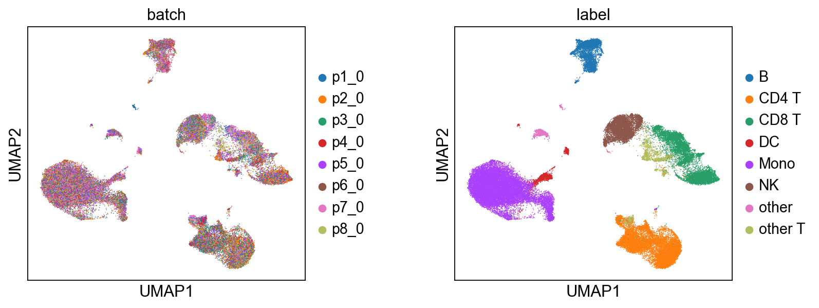
6.1 Joint Embeddings

# Biological State (z_c) — coloured by batch and cell type.
scmidas.pl.umap(
    mdata, basis='X_midas',
    color=['batch', 'label'], wspace=0.4,
)
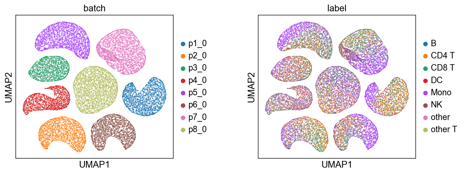
# Technical Noise (z_u)
scmidas.pl.umap(
    mdata, basis='X_midas_u',
    color=['batch', 'label'], wspace=0.4,
)

AnnData object with n_obs × n_vars = 52964 × 2
    obs: 'label', 'batch'
    uns: 'neighbors', 'umap', 'batch_colors', 'label_colors'
    obsm: 'X_umap'
    obsp: 'distances', 'connectivities'

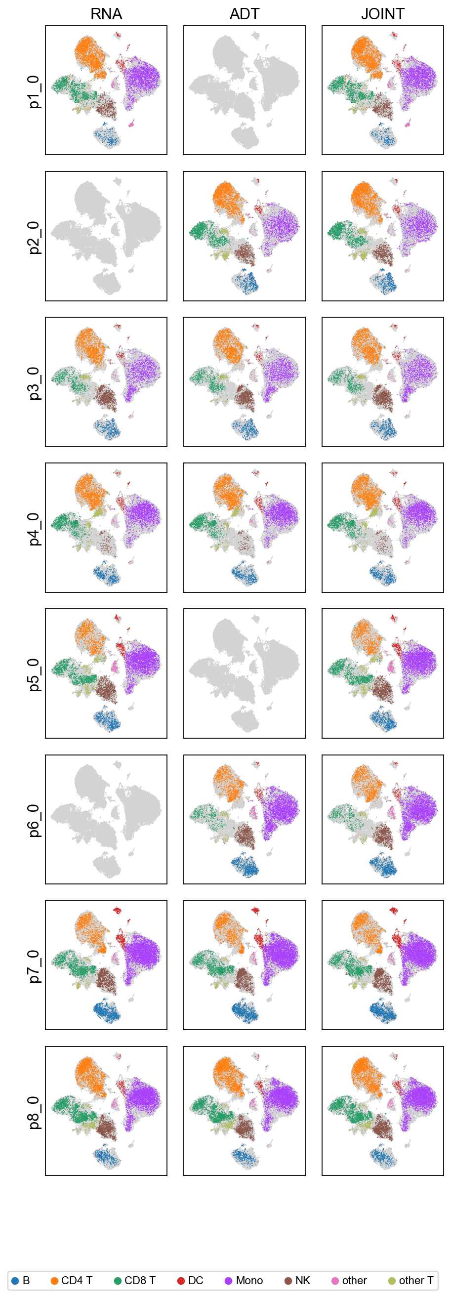
6.2 Modality-Specific Embeddings

We visualize the biological embeddings (c) for each modality (RNA, ADT) and for the joint representation, across all 8 batches.

# Per-modality biological latent grid (modality × batch),
# coloured by cell type. Internally re-runs predict(mod_latent=True);
# the per-modality views answer 'does this single modality alone
# carry enough signal to separate cell types in this batch?'
scmidas.pl.modality_grid(model, mdata, label_key='label')

AnnData object with n_obs × n_vars = 133603 × 32
    obs: 'type', 'batch', 'label'
    uns: 'neighbors', 'umap', 'label_colors'
    obsm: 'X_umap'
    obsp: 'distances', 'connectivities'

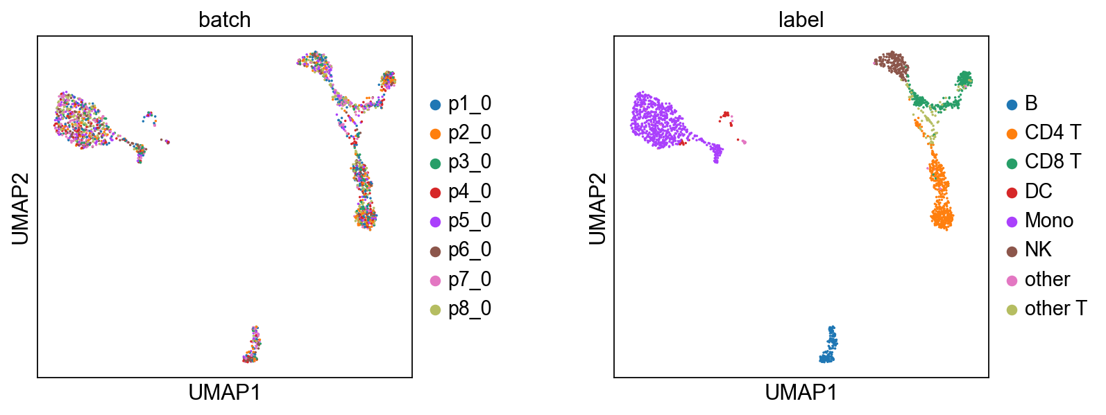
6.3 Imputed and Batch-Corrected Data

We use WNN to compute joint embeddings from the imputed and batch-corrected counts.

For efficiency, we’ll use a random sample of 2000 cells.

N = 2000
select = np.random.choice(list(range(len(adata))), N, replace=False)
data = {
    'x_bc_rna' : adata.obsm['x_bc_rna'][select],
    'x_bc_adt' : adata.obsm['x_bc_adt'][select],
}

We subsample the imputed and batch-corrected data, save them to disk, execute the R script to perform WNN and UMAP, and then load and plot the results.

temp_dirs = {"Imputed and Batch-Corrected Data": 'demo2_temp/x_bc/'}
r_script_file = 'wnn_bimodal.R' # R script for WNN analysis on RNA+ADT data
download_script(r_script_file)

for name, temp_dir in temp_dirs.items():
    # 1. Save Python data to disk for the R script to access
    os.makedirs(temp_dir, exist_ok=True)
    data_key = Path(temp_dir).name  # 'x_bc' or 'x'
    pd.DataFrame(data[data_key+'_rna']).T.to_csv(temp_dir+'rna.csv', index=True)
    pd.DataFrame(data[data_key+'_adt']).T.to_csv(temp_dir+'adt.csv', index=True)

    # 2. Execute the R script via a subprocess
    print(f"\nPython: Executing R script '{r_script_file}' for {name}...\n")
    command = ['Rscript', '--vanilla', r_script_file, temp_dir]
    result = subprocess.run(command, check=True, capture_output=True, text=True)
    # print(result.stdout) # uncomment this line to see the R script's output

    # 3. Load the UMAP results generated by R and plot them
    ad = adata[select]
    ad.obsm['umap'] = pd.read_csv(temp_dir+'umap_coords.csv', index_col=0).values
    # shuffle
    sc.pp.subsample(ad, fraction=1)
    sc.pl.umap(ad, color=['batch', 'label'], size=10, wspace=0.4)

'wnn_bimodal.R' already exists. Skipping download.

Python: Executing R script 'wnn_bimodal.R' for Imputed and Batch-Corrected Data...

... storing 'batch' as categorical
... storing 'label' as categorical

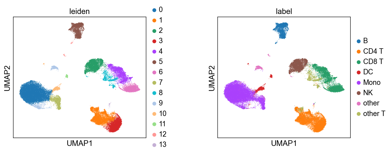
6.4 After integration: clustering and visualization

Once mdata.obsm['X_midas'] is populated, MIDAS is out of the picture — the rest is generic single-cell analysis. Here we cluster with Leiden on the integrated representation and compare against the published cell-type labels. For automated cell-type calling, CellTypist plugs in directly here.

# Run Leiden on the integrated latent. We wrap mdata.obsm['X_midas'] as an
# AnnData for the cluster step (Leiden takes AnnData), then carry the labels
# back to the MuData for plotting via scmidas.pl.umap.
import anndata as ad
ad_view = ad.AnnData(X=mdata.obsm['X_midas'], obs=mdata.obs[['batch', 'label']].copy())
sc.pp.neighbors(ad_view, use_rep='X', n_neighbors=15)
sc.tl.leiden(ad_view, resolution=0.5)
mdata.obs['leiden'] = ad_view.obs['leiden'].values

# Side-by-side: Leiden clusters from MIDAS-integrated data vs. ground-truth labels.
scmidas.pl.umap(mdata, basis='X_midas', color=['leiden', 'label'], wspace=0.4)

AnnData object with n_obs × n_vars = 52964 × 32
    obs: 'leiden', 'label'
    uns: 'leiden_colors', 'label_colors'
    obsm: 'X_umap'