Rectangular Integration of RNA+ADT

In this tutorial, we demonstrate how to use MIDAS to integrate a rectangular dataset consisting of paired RNA (gene expression) and ADT (antibody-derived tags) data. We will walk through the entire process, from data setup and model training to inference and evaluation of the results.

1. Setting Up the Environment

We import the necessary libraries and set up the environment. The first code cell exposes a small GPU configuration block — GPUS and STRATEGY — that controls which device(s) the demo uses. The defaults run on a single GPU; switching to multi-GPU only requires changing those two values (see the comments inside that cell).

import warnings
warnings.filterwarnings('ignore')
import logging
logging.basicConfig(level=logging.INFO)
import os

# === GPU configuration ===
# Single-GPU (default; works inside this notebook):
GPUS = '0'
STRATEGY = 'auto'

# Multi-GPU options (uncomment one):
# - In a notebook (slower DDP startup, no script conversion needed):
#       GPUS = '0,1'; STRATEGY = 'ddp_notebook'
# - As a script (recommended for production multi-GPU):
#       GPUS = '0,1'; STRATEGY = 'ddp'
#       Run with: jupyter nbconvert --to script <this notebook>.ipynb && python <this notebook>.py

if GPUS is not None:
    os.environ['CUDA_VISIBLE_DEVICES'] = GPUS

# Lightning's `devices='auto'` defaults to 1 in notebooks even when more GPUs
# are visible, so we derive an explicit device count from `GPUS`.
DEVICES = len(GPUS.split(',')) if GPUS else 'auto'
# === /GPU configuration ===

import subprocess
from pathlib import Path

import lightning as L
import numpy as np
import pandas as pd
import scanpy as sc

from scmidas.config import load_config
from scmidas.data import download_data, download_models, download_script
import scmidas

sc.set_figure_params(figsize=(4, 4))    # Set plotting parameters for scanpy
L.seed_everything(42)                   # Set a global random seed for reproducibility

INFO: Seed set to 42
INFO:lightning.fabric.utilities.seed:Seed set to 42

42

2. Downloading the Data

We will use a public dataset for this demonstration. The task variable defines the dataset name, which corresponds to a multi-batch (8 batches) RNA+ADT dataset in mtx format. The download_data function will automatically fetch and place it in the dataset/ directory.

task = 'wnn_full_8batch_mtx'
download_data(task)

# Load directory-format dataset as a MuData (one AnnData per modality).
mdata = scmidas.datasets.from_dir(
    f'dataset/{task}/data',
    label_dir=f'dataset/{task}/label',
)
mdata

INFO:scmidas.data:Downloading from https://pub-cfde59ed245349228f47377c9ae32dd3.r2.dev/wnn_full_8batch_mtx.zip.
Downloading wnn_full_8batch_mtx.zip: 100%|██████████| 114M/114M [00:08<00:00, 13.8MB/s]
INFO:scmidas.data:Downloaded: https://pub-cfde59ed245349228f47377c9ae32dd3.r2.dev/wnn_full_8batch_mtx.zip to dataset/wnn_full_8batch_mtx.zip
INFO:scmidas.data:Unzipped: dataset/wnn_full_8batch_mtx.zip to dataset
INFO:scmidas.datasets:from_dir: loaded 2 modalities (['rna', 'adt']) across 8 batches.

MuData object with n_obs × n_vars = 52964 × 3841
  obs:      'batch', 'label'
  uns:      'feat_dims'
  2 modalities
    rna:    52964 × 3617
      obs:  'batch', 'label'
      uns:  'mask_p1_0', 'mask_p2_0', 'mask_p3_0', 'mask_p4_0', 'mask_p5_0', 'mask_p6_0', 'mask_p7_0', 'mask_p8_0'
    adt:    52964 × 224
      obs:  'batch', 'label'
      uns:  'mask_p1_0', 'mask_p2_0', 'mask_p3_0', 'mask_p4_0', 'mask_p5_0', 'mask_p6_0', 'mask_p7_0', 'mask_p8_0'

3. Configuring the Model

Next, we configure the MIDAS model. We start by loading the default configuration, which contains optimized hyperparameters for various tasks. We then instruct the model where to find the data and where to save the trained model artifacts.

configs = load_config()
configs['num_workers'] = 8  # Adjust based on your system's CPU cores for data loading

scmidas.MIDAS.setup_mudata(mdata, batch_key='batch')
model = scmidas.MIDAS(
    mdata,
    configs=configs,
    save_model_path=f'saved_models/{task}',
)

INFO:scmidas.config:The model is initialized with the default configurations.
INFO:scmidas.model:setup_mudata: batch_key='batch', batches=['p1_0', 'p2_0', 'p3_0', 'p4_0', 'p5_0', 'p6_0', 'p7_0', 'p8_0'], modalities=['rna', 'adt'], dims_x={'rna': [3617], 'adt': [224]}
INFO:scmidas.model:Input data:
      #CELL  #RNA  #ADT  #VALID_RNA  #VALID_ADT
p1_0   6378  3617   224      3617.0       224.0
p2_0   5899  3617   224      3617.0       224.0
p3_0   4628  3617   224      3617.0       224.0
p4_0   5285  3617   224      3617.0       224.0
p5_0   6952  3617   224      3617.0       224.0
p6_0   6060  3617   224      3617.0       224.0
p7_0   8854  3617   224      3617.0       224.0
p8_0   8908  3617   224      3617.0       224.0

4. Training the Model

We have two options: use a pre-trained model for a quick start or train the model from scratch to see the full process. For this demo, we will use the pre-trained version. To train from scratch, simply set use_pretrained = False.

use_pretrained = True # To train from scratch, set it to False

if use_pretrained:
    download_models(task)
    model.load_checkpoint(f'saved_models/{task}.pt')
else:
    model.train(
        max_epochs=1500,
        accelerator='gpu',
        devices=DEVICES,
        strategy=STRATEGY,
    )

INFO:scmidas.data:Downloading from https://pub-cfde59ed245349228f47377c9ae32dd3.r2.dev/wnn_full_8batch_mtx.pt.
Downloading wnn_full_8batch_mtx.pt: 100%|██████████| 98.5M/98.5M [00:21<00:00, 4.56MB/s]
INFO:scmidas.data:Downloaded: https://pub-cfde59ed245349228f47377c9ae32dd3.r2.dev/wnn_full_8batch_mtx.pt to saved_models/wnn_full_8batch_mtx.pt

5. Generating Predictions

With a trained model, MIDAS exposes two prediction surfaces:

• High-level (recommended): model.get_latent_representation(kind='c'|'u'|'joint') and model.get_imputed_values(modality=...) return aligned arrays writable straight into mdata.obsm.

• Low-level (advanced): model.predict(...) exposes every flag (per-modality latents, modality translation, batch-corrected reconstructions). Used below for visualizations that need the per-modality and batch-corrected outputs.

# High-level API — write joint latents to mdata.obsm
mdata.obsm['X_midas']   = model.get_latent_representation(kind='c')          # biological c (32-dim)
mdata.obsm['X_midas_u'] = model.get_latent_representation(kind='u')          # technical u (2-dim)
print('mdata.obsm[X_midas].shape   =', mdata.obsm['X_midas'].shape)
print('mdata.obsm[X_midas_u].shape =', mdata.obsm['X_midas_u'].shape)

mdata.obsm[X_midas].shape   = (52964, 32)
mdata.obsm[X_midas_u].shape = (52964, 2)

outputs = model.predict(
        joint_latent=True,
        input=True,
        batch_correct=True,
        impute=True,
        translate=True,
        mod_latent=True,
        )

INFO:scmidas.model:Predicting using device: cuda
INFO:scmidas.model:Processing batch p1_0: ['rna', 'adt']
predict:p1_0: 100%|██████████| 25/25 [00:01<00:00, 22.68it/s]
INFO:scmidas.model:Processing batch p2_0: ['rna', 'adt']
predict:p2_0: 100%|██████████| 24/24 [00:01<00:00, 20.99it/s]
INFO:scmidas.model:Processing batch p3_0: ['rna', 'adt']
predict:p3_0: 100%|██████████| 19/19 [00:00<00:00, 21.48it/s]
INFO:scmidas.model:Processing batch p4_0: ['rna', 'adt']
predict:p4_0: 100%|██████████| 21/21 [00:01<00:00, 20.37it/s]
INFO:scmidas.model:Processing batch p5_0: ['rna', 'adt']
predict:p5_0: 100%|██████████| 28/28 [00:01<00:00, 23.30it/s]
INFO:scmidas.model:Processing batch p6_0: ['rna', 'adt']
predict:p6_0: 100%|██████████| 24/24 [00:01<00:00, 18.22it/s]
INFO:scmidas.model:Processing batch p7_0: ['rna', 'adt']
predict:p7_0: 100%|██████████| 35/35 [00:01<00:00, 23.28it/s]
INFO:scmidas.model:Processing batch p8_0: ['rna', 'adt']
predict:p8_0: 100%|██████████| 35/35 [00:01<00:00, 23.36it/s]
INFO:scmidas.model:Batch correction (second pass) ...
INFO:scmidas.model:Processing batch p1_0: ['rna', 'adt']
batch_correct:p1_0: 100%|██████████| 25/25 [00:01<00:00, 24.87it/s]
INFO:scmidas.model:Processing batch p2_0: ['rna', 'adt']
batch_correct:p2_0: 100%|██████████| 24/24 [00:01<00:00, 23.99it/s]
INFO:scmidas.model:Processing batch p3_0: ['rna', 'adt']
batch_correct:p3_0: 100%|██████████| 19/19 [00:00<00:00, 19.39it/s]
INFO:scmidas.model:Processing batch p4_0: ['rna', 'adt']
batch_correct:p4_0: 100%|██████████| 21/21 [00:00<00:00, 21.13it/s]
INFO:scmidas.model:Processing batch p5_0: ['rna', 'adt']
batch_correct:p5_0: 100%|██████████| 28/28 [00:01<00:00, 21.05it/s]
INFO:scmidas.model:Processing batch p6_0: ['rna', 'adt']
batch_correct:p6_0: 100%|██████████| 24/24 [00:01<00:00, 17.79it/s]
INFO:scmidas.model:Processing batch p7_0: ['rna', 'adt']
batch_correct:p7_0: 100%|██████████| 35/35 [00:01<00:00, 27.41it/s]
INFO:scmidas.model:Processing batch p8_0: ['rna', 'adt']
batch_correct:p8_0: 100%|██████████| 35/35 [00:01<00:00, 30.89it/s]

ad_list = []
for k, v in outputs.items():
    ad = sc.AnnData(np.zeros([v['s']['joint'].shape[0], 1]))
    for var in ['z_c', 'z_u', 'x_bc', 'x']:
        for m in v[var].keys():
            ad.obsm['%s_%s'%(var,m)] = v[var][m]
    ad.obs['batch'] = k
    ad.obs['label'] = pd.read_csv('./dataset/'+task+'/label/%s.csv'%k, index_col=0).values.flatten()
    ad_list.append(ad)

adata = sc.concat(ad_list)
adata

AnnData object with n_obs × n_vars = 52964 × 1
    obs: 'batch', 'label'
    obsm: 'z_c_joint', 'z_c_rna', 'z_c_adt', 'z_u_joint', 'z_u_rna', 'z_u_adt', 'x_bc_rna', 'x_bc_adt', 'x_rna', 'x_adt'

6. Visualizing the Results

Now, let’s visualize the outputs to assess the model’s performance. First, we need to load the cell-type labels and batch identifiers for annotation.

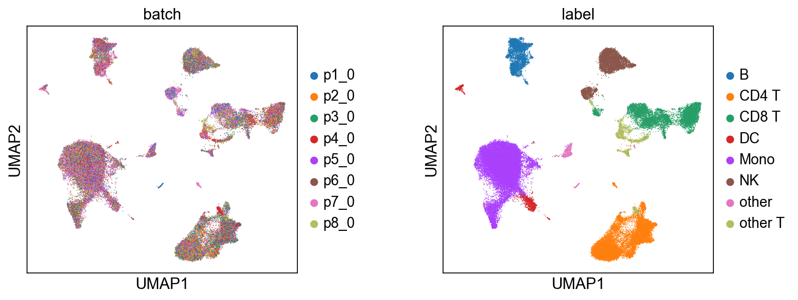
6.1 Joint Embeddings

We infer the joint embedding z, which is composed of a biological component c and a technical component u.

# Biological State (z_c) — coloured by batch and cell type.
scmidas.pl.umap(
    mdata, basis='X_midas',
    color=['batch', 'label'], wspace=0.4,
)
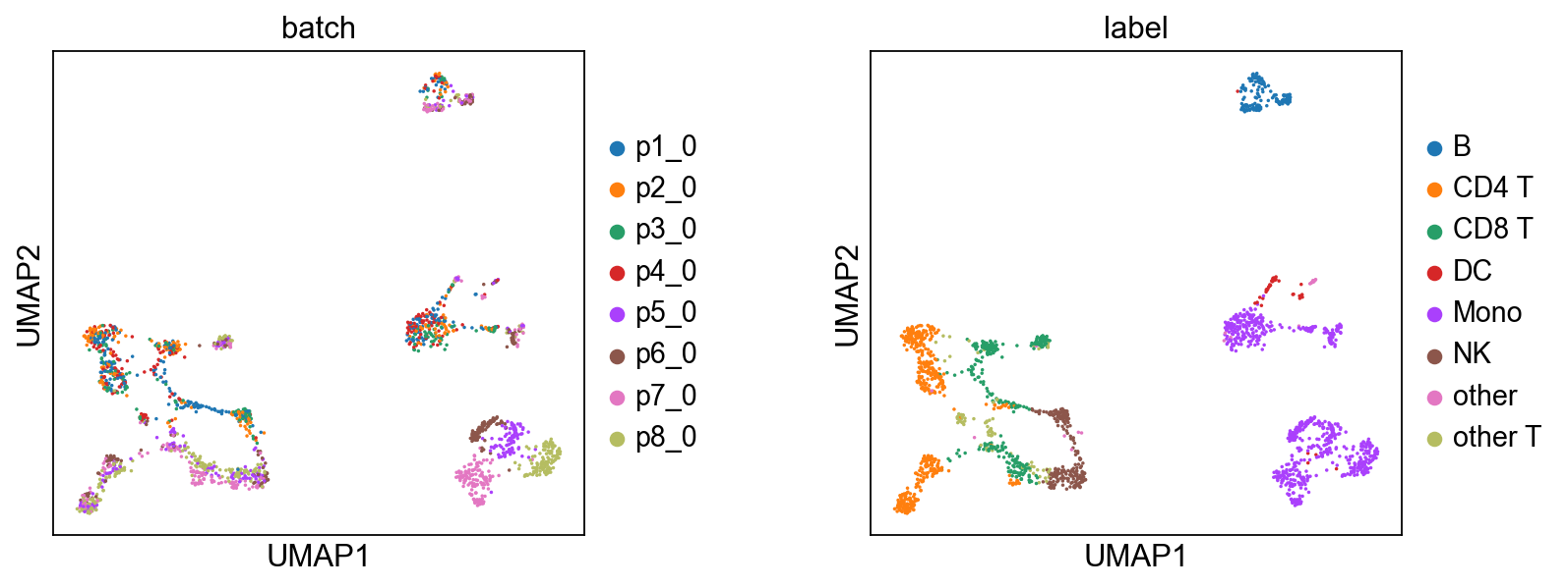
# Technical Noise (z_u)
scmidas.pl.umap(
    mdata, basis='X_midas_u',
    color=['batch', 'label'], wspace=0.4,
)

AnnData object with n_obs × n_vars = 52964 × 2
    obs: 'label', 'batch'
    uns: 'neighbors', 'umap', 'batch_colors', 'label_colors'
    obsm: 'X_umap'
    obsp: 'distances', 'connectivities'

6.2 Modality-Specific Embeddings

Here, we visualize the biological embeddings (c) for each modality (RNA, ADT) and for the joint representation, across all 8 batches. This helps us understand how well-aligned the different modalities are within each batch after being projected into the common latent space.

# Per-modality biological latent grid (modality × batch),
# coloured by cell type. Internally re-runs predict(mod_latent=True);
# the per-modality views answer 'does this single modality alone
# carry enough signal to separate cell types in this batch?'
scmidas.pl.modality_grid(model, mdata, label_key='label')

AnnData object with n_obs × n_vars = 158892 × 32
    obs: 'type', 'batch', 'label'
    uns: 'neighbors', 'umap', 'label_colors'
    obsm: 'X_umap'
    obsp: 'distances', 'connectivities'

6.3 Batch-Corrected Data vs. Original Data

To externally validate the quality of MIDAS’s batch-corrected count data, we will use a third-party algorithm, Seurat’s Weighted Nearest Neighbor (WNN), to compute joint embeddings from both the batch-corrected and original counts.

For efficiency, we’ll use a random sample of 2000 cells for the comparison.

N = 2000
select = np.random.choice(list(range(len(adata))), N, replace=False)
data = {
    'x_bc_rna' : adata.obsm['x_bc_rna'][select],
    'x_bc_adt' : adata.obsm['x_bc_adt'][select],
    'x_rna' : adata.obsm['x_rna'][select],
    'x_adt' : adata.obsm['x_adt'][select],
}

Now, we will loop through the batch-corrected and original data. For each, we save the subsampled data to disk, execute the R script to perform WNN and UMAP, and then load and plot the results.

temp_dirs = {"Batch-Corrected Data": 'demo1_temp/x_bc/', "Original Data": 'demo1_temp/x/'}
r_script_file = 'wnn_bimodal.R' # R script for WNN analysis on RNA+ADT data
download_script(r_script_file)

for name, temp_dir in temp_dirs.items():
    # 1. Save Python data to disk for the R script to access
    os.makedirs(temp_dir, exist_ok=True)
    data_key = Path(temp_dir).name  # 'x_bc' or 'x'
    pd.DataFrame(data[data_key+'_rna']).T.to_csv(temp_dir+'rna.csv', index=True)
    pd.DataFrame(data[data_key+'_adt']).T.to_csv(temp_dir+'adt.csv', index=True)

    # 2. Execute the R script via a subprocess
    # print(f"\nPython: Executing R script '{r_script_file}' for {name}...\n")
    command = ['Rscript', '--vanilla', r_script_file, temp_dir]
    result = subprocess.run(command, check=True, capture_output=True, text=True)
    print(result.stdout) # uncomment this line to see the R script's output

    # 3. Load the UMAP results generated by R and plot them
    ad = adata[select]
    ad.obsm['umap'] = pd.read_csv(temp_dir+'umap_coords.csv', index_col=0).values
    # shuffle
    sc.pp.subsample(ad, fraction=1)
    sc.pl.umap(ad, color=['batch', 'label'], size=10, wspace=0.4)

'wnn_bimodal.R' already exists. Skipping download.

... storing 'batch' as categorical
... storing 'label' as categorical

[1] "R script: Reading data..."
[1] "R script: Creating Seurat object..."
An object of class Seurat
3841 features across 2000 samples within 2 assays
Active assay: rna (3617 features, 0 variable features)
 1 other assay present: adt
[1] "R script: Running RNA processing..."
[1] "R script: Running ADT processing..."
[1] "R script: Running WNN..."
[1] "R script: Running UMAP..."
[1] "R script: Finished."

... storing 'batch' as categorical
... storing 'label' as categorical

[1] "R script: Reading data..."
[1] "R script: Creating Seurat object..."
An object of class Seurat
3841 features across 2000 samples within 2 assays
Active assay: rna (3617 features, 0 variable features)
 1 other assay present: adt
[1] "R script: Running RNA processing..."
[1] "R script: Running ADT processing..."
[1] "R script: Running WNN..."
[1] "R script: Running UMAP..."
[1] "R script: Finished."

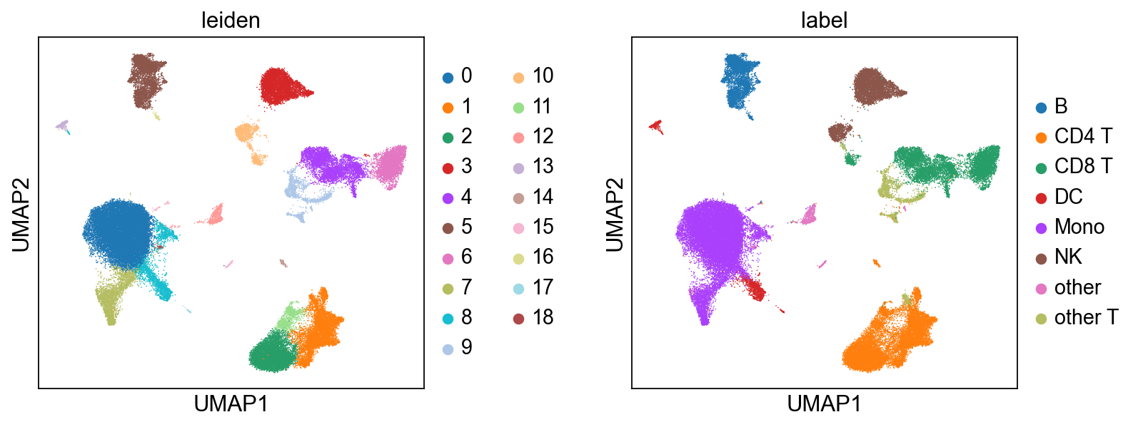
6.4 After integration: clustering and visualization

Once mdata.obsm['X_midas'] is populated, MIDAS is out of the picture — the rest is generic single-cell analysis. Here we cluster with Leiden on the integrated representation and compare against the published cell-type labels. For automated cell-type calling, CellTypist plugs in directly here.

# Run Leiden on the integrated latent. We wrap mdata.obsm['X_midas'] as an
# AnnData for the cluster step (Leiden takes AnnData), then carry the labels
# back to the MuData for plotting via scmidas.pl.umap.
import anndata as ad
ad_view = ad.AnnData(X=mdata.obsm['X_midas'], obs=mdata.obs[['batch', 'label']].copy())
sc.pp.neighbors(ad_view, use_rep='X', n_neighbors=15)
sc.tl.leiden(ad_view, resolution=0.5)
mdata.obs['leiden'] = ad_view.obs['leiden'].values

# Side-by-side: Leiden clusters from MIDAS-integrated data vs. ground-truth labels.
scmidas.pl.umap(mdata, basis='X_midas', color=['leiden', 'label'], wspace=0.4)

AnnData object with n_obs × n_vars = 52964 × 32
    obs: 'leiden', 'label'
    uns: 'leiden_colors', 'label_colors'
    obsm: 'X_umap'